Real-Time Equilibrium Reconstruction

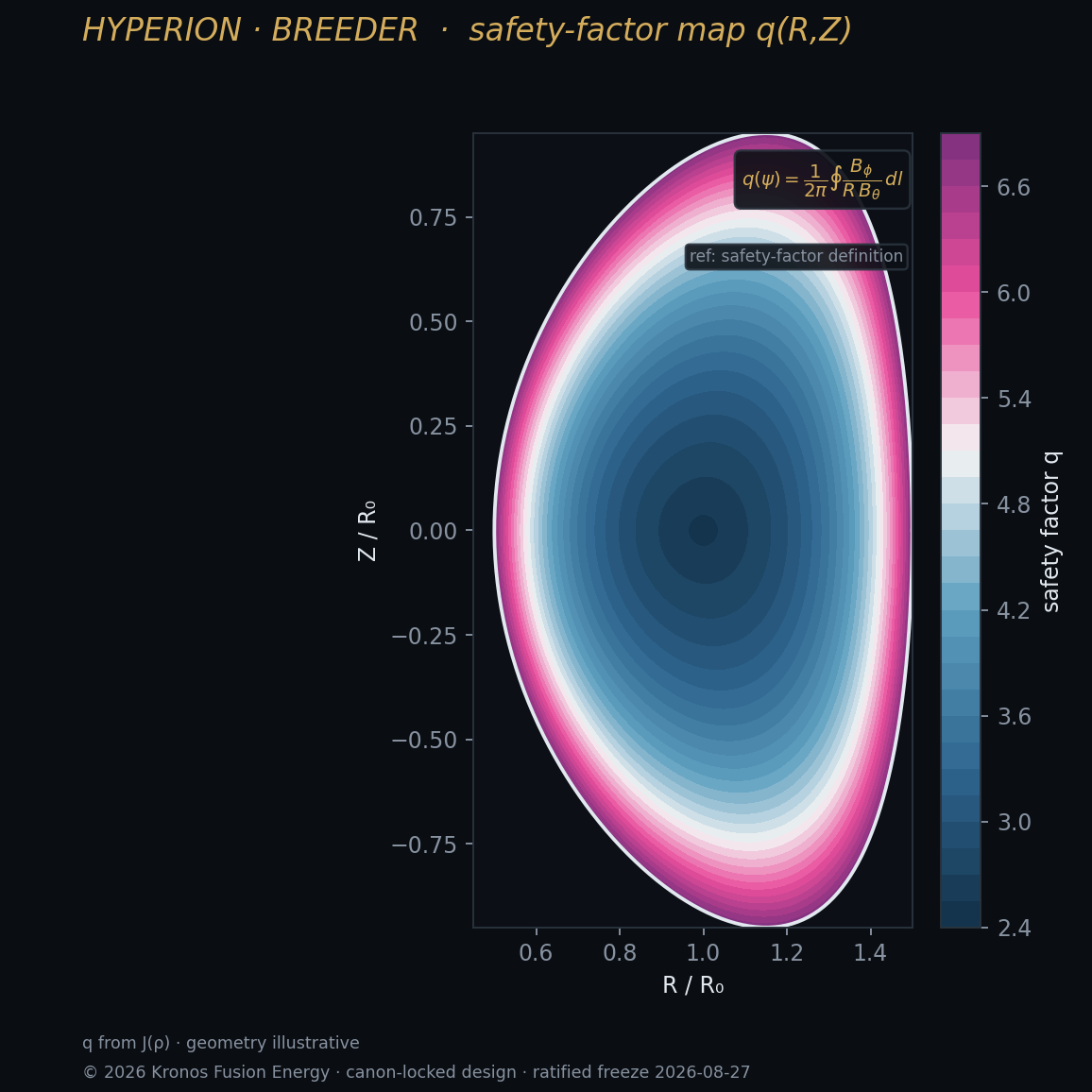
L1 solves a fast, bounded Grad-Shafranov reconstruction each cycle to give the shape and position loops a physically consistent state estimate.

Why reconstruct in real time

Shape, position, and current loops all act on the plasma equilibrium, but the equilibrium is not directly measured — it is inferred from magnetics. L1 runs a fast equilibrium reconstruction every control cycle, solving a reduced form of the Grad-Shafranov equation constrained by the measured flux loops and Mirnov coils, to produce a consistent boundary, position, and moment set.

The Grad-Shafranov constraint

In axisymmetric equilibrium the poloidal flux ψ satisfies the Grad-Shafranov equation, R ∂/∂R((1/R)∂ψ/∂R) + ∂²ψ/∂z² = −μ0 R² p'(ψ) − FF'(ψ). The full solve is nonlinear and iterative; the fast in-loop version is bounded — a fixed number of iterations or a linearized update — so its WCET is known. The high-fidelity reconstruction runs at L3 as the digital twin's equilibrium module.

Bounded computation

• Fixed iteration cap with a defined fallback for the fast solve.
• Fixed-point arithmetic with analyzed word growth in fabric.
• Outputs: boundary moments, R, z, I_p-consistent flux state.
• Validity mask propagated from the diagnostics that feed it.

The design accepts a slightly lower-fidelity but strictly-timed estimate in the fast loop, because a controller needs a consistent answer on time more than a perfect answer late. The twin's richer reconstruction corrects and audits the fast estimate on the 50–100 ms shadow horizon.

PINN acceleration

Kronos's L3 uses physics-informed neural networks (PINNs) trained to satisfy Grad-Shafranov, which can produce equilibria far faster than iterative solvers. Their role is to sharpen the advisory target and the twin, not to sit in the deterministic loop; the fast in-fabric solve remains the certified estimator that the shape and stability loops depend on.