Flux-Coordinate Normalization

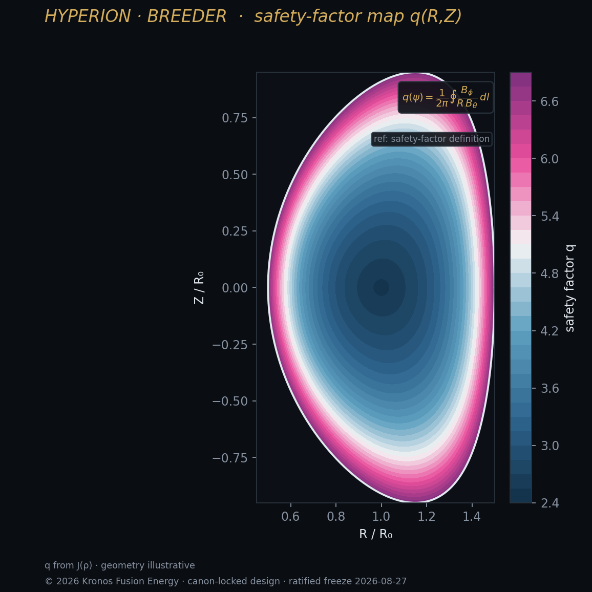
Mapping breeder diagnostics onto normalized poloidal flux makes profiles shot-invariant and gives the equilibrium PINN its natural coordinate.

Normalized flux as the ruler

In the breeder (Hyperion), the confinement geometry is set by nested flux surfaces. Normalized poloidal flux psi_N runs from 0 on the magnetic axis to 1 at the last closed flux surface. Expressing every profile diagnostic against psi_N — rather than against machine radius — removes the ambiguity introduced when the plasma shifts, breathes, or changes its negative-triangularity shape (delta -0.30).

Why the shape makes this hard

Negative triangularity pulls the outboard edge inward, and at aspect ratio 2.5 the flux surfaces are strongly shaped. A naive radial mapping would misplace edge diagnostics badly. The normalization uses the reconstructed equilibrium to place each sample on the correct surface, so an edge pressure sample lands at the right psi_N even as the boundary moves shot to shot.

Coupled to the equilibrium solver

Flux-coordinate normalization and equilibrium reconstruction are mutually dependent: the mapping needs the equilibrium, and the equilibrium fit uses normalized magnetics. The fabric provides a fast, calibrated first mapping from magnetics; the L3 PINN that solves Grad-Shafranov then refines it. The fabric records which equilibrium version produced a given normalization.

# place a profile sample on a flux surface
def to_psi_n(R, Z, equilibrium):
    psi   = equilibrium.psi(R, Z)          # interpolated flux
    psi_n = (psi - equilibrium.psi_axis) / (
             equilibrium.psi_lcfs - equilibrium.psi_axis)
    return max(0.0, min(1.0, psi_n))

Payoff

• Profiles become comparable across shots, enabling clean feature stores and training sets.
• The core pressure map and instantaneous Q are computed in the frame the physics lives in.
• Edge diagnostics for the ELM-free negative-triangularity regime are correctly localized.